Understanding Database Indexing
The primary goal of a database system is to store data efficiently and provide quick access to it. Instead of relying on filesystem hierarchies, database systems use specialized file organization for three key reasons:
- Storage efficiency: Minimize storage overhead per record
- Access efficiency: Locate records in the smallest number of steps
- Update efficiency: Minimize disk changes when updating records
How Data is Organized
Database systems store data as records (rows with multiple fields) in tables. Each record can be looked up using a search key. To do this efficiently, databases use indexes: a data structure technique that improves the speed of data retrieval O(log N) or even O(1) by minimizing disk accesses without scanning an entire table on every access.
Index Data Structure: B-Tree (Balanced Tree)
The most common index structure is a B-Tree, the default index type (always on primary keys by default). It maintains a sorted tree structure where the “Root” points to “Branches,” which point to “Leaves” (where the actual data pointers are).
Best For: Exact matches (=) and range queries (>, <, BETWEEN).
Complexity: O(log N).
Why Range Queries Work: If you want IDs > 7, the database finds 20, then just reads the “next” pointers (11, 13, 17, …) sequentially without traversing the tree again.
Used by: Most relational databases (MySQL, PostgreSQL, Oracle) as the default index structure.
Two Data Storage Approaches
1. Index-Organized Storage (Clustered Index)
In this approach, data lives inside the index itself. Leaf nodes of the B+ tree store full rows, so no separate heap file exists.
B+ Tree Structure:
  leaf: key → full row
Query execution: Traverse the index and the row is already there (single lookup).
Advantages: Fast primary-key lookups, excellent range queries, good cache locality.
Used by: MySQL InnoDB (primary key), Oracle IOT, SQL Server clustered index.
2. Heap-Organized Table + Separate Index (Most Common)
Rows are stored unsorted in a heap, and the index is a separate structure that points to them.
Index (B+ Tree):    key → (page, slot)
Heap Data File:     page → record
Query execution: (1) Search the index, (2) Follow the pointer, (3) Read the data page (two lookups).
Advantages: Fast inserts, fast updates, flexible storage.
Disadvantages: Extra I/O overhead, poor range query locality.
Used by: PostgreSQL, SQL Server (non-clustered indexes).
When to Use Each Approach
No single strategy is optimal for all workloads:
| Workload | Best Choice |
|---|---|
| Heavy inserts | Heap |
| Frequent updates | Heap |
| Range queries | Clustered |
| Read-heavy OLTP | Clustered |
| Mixed workload | Heap + indexes |
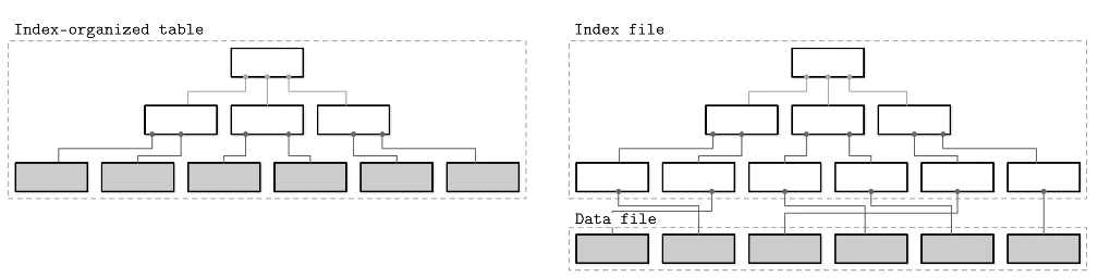
Visual comparison of index-organized storage (left) where data is stored within the index structure itself, versus heap-organized storage with a separate index file pointing to a data file (right).
Secondary Indexes: When the Primary Index Isn’t Enough
Even if data is stored in a clustered index, queries often search on non-clustered columns. For example:
SELECT * FROM users WHERE email = 'a@gmail.com';If the data is clustered (sorted) by user_id, the clustered index is useless for this query. The database needs a secondary index on the email column.
Without a Secondary Index
The database must perform a Clustered Index Scan (or table scan): start at the first leaf page, read every row, check each email value, and stop only at the end. This is O(N) complexity—very slow.
With a Secondary Index
A secondary index on email stores:
email → user_id (or reference to row)Query execution:
- Search the secondary index (B+ tree) for
'a@gmail.com'→ getuser_id = 3 - Use the primary/clustered index on
user_idto fetch the row
This Index Seek + Key Lookup is approximately O(log N)—much faster.
Key insight: Only ONE index can define physical storage (the clustered index). All other indexes are secondary indexes that must somehow reference the data.
Two Approaches for Secondary Index Implementation
Secondary indexes can reference data in two fundamentally different ways, each with different performance trade-offs:
Approach A: Direct References (RID-based)
Secondary indexes store direct pointers to data:
Secondary index: key → (PageID, SlotID)Lookup path: Secondary Index → Data Page (direct jump, single lookup).
Advantages: Faster reads (fewer lookups), fewer tree traversals.
Disadvantages: If rows move (due to page splits, compaction, or vacuum operations), ALL secondary indexes must be updated. This becomes very expensive with many indexes.
Used by: PostgreSQL, older database designs, systems optimized for read performance.
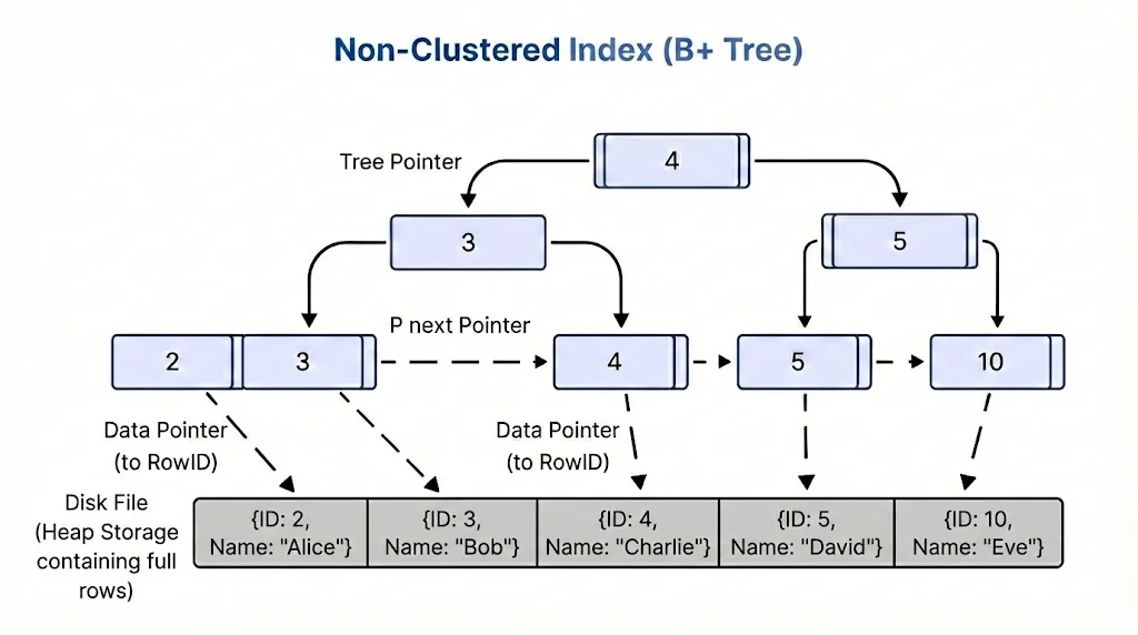
How a non-clustered B+ tree index uses direct data pointers (RowIDs) to locate rows in the heap file. Each leaf node contains index keys and direct pointers to the corresponding row locations, enabling single-step data access after finding the key.
Approach B: Indirection via Primary Index (PK-based)
Secondary indexes store references to the primary key:
Secondary index: secondary_key → primary_key
Primary index:   primary_key → actual row
Lookup path: Secondary Index → Primary Index → Data (two lookups).
Why this indirection? When rows move (due to page splits, reorganization, or background maintenance), only the primary index is updated—secondary indexes stay untouched. This massively reduces write amplification in write-heavy systems.
Used by: MySQL InnoDB (the most common modern approach).
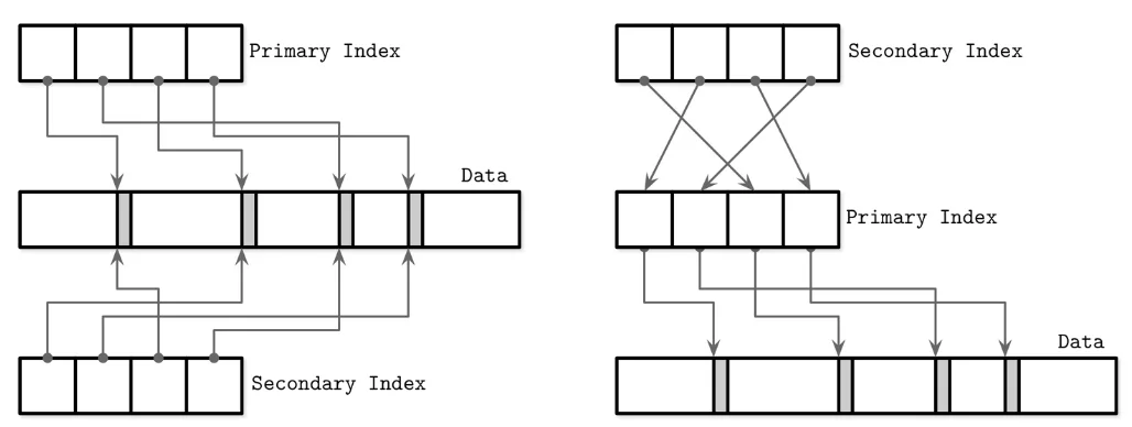
How secondary indexes reference the primary index instead of data directly. Secondary indexes point to primary key values, which then point to actual data. This reduces write amplification when rows move.
The Trade-off (The Key Insight)
| Strategy | Read Cost | Write Cost |
|---|---|---|
| Direct pointer | Low | High |
| PK indirection | Higher | Lower |
- Read-heavy workload? Direct pointers are acceptable.
- Write-heavy workload or many indexes? PK indirection wins by avoiding expensive updates to every index.
Concrete MySQL InnoDB Example
SELECT * FROM users WHERE email = 'a@gmail.com';InnoDB execution (using PK indirection):
- Search secondary index on
email→ find'a@gmail.com'→ getuser_id = 3 - Search the primary (clustered) index on
user_id - Fetch the row
This demonstrates how secondary indexes point to primary keys, not directly to data. The indirection adds a lookup but greatly reduces write overhead when rows move.
Alternative Index Structures
While B-Trees are the default, different scenarios require different index structures for specialized use cases:
Hash Index
Concept: Uses a mathematical formula (hash function) to calculate a specific memory slot (bucket) for a key.
Best For: Exact lookups only (WHERE name = ‘Alice’).
Limitation: No range queries. The physical storage order is random.
Example:
Query: WHERE name = 'Alice'
Hash Function: Hash('Alice') = Bucket 003

Key        Hash Calculation    Storage Bucket
'Alice'    func('Alice')       Bucket 003
'Bob'      func('Bob')         Bucket 052
'Charlie'  func('Charlie')     Bucket 001

Memory Layout:
[Bucket 001] → Charlie's Data
[Bucket 002] → (Empty)
[Bucket 003] → Alice's Data  ← Direct jump here! (O(1))
...
[Bucket 052] → Bob's Data
Why Ranges Fail: Notice that Alice (A) is in Bucket 3, but Bob (B) is in Bucket 52. They are not adjacent, so the database cannot scan for “Names from A to B.”
Used by: MySQL MEMORY table engine, some NoSQL databases for exact lookups.
C. Bitmap Index
Concept: Uses bit arrays (0s and 1s) for columns with low cardinality (few unique values).
Best For: Gender, Marital Status, Is_Active, or any column with limited distinct values.
Pros: Ultra-fast bitwise operations (AND, OR, NOT) with minimal memory overhead.
Example:
Table Data (4 Rows):
1. Male, Single
2. Female, Married
3. Female, Single
4. Male, Married

Bitmap Index Representation:
Row ID    Gender='Male'    Gender='Female'    Status='Single'    Status='Married'
1         1                0                  1                  0
2         0                1                  0                  1
3         0                1                  1                  0
4         1                0                  0                  1

Finding "Female AND Single":
CPU compares bits:
0 1 1 0 (Female Vector)
1 0 1 0 (Single Vector)
AND -------
0 0 1 0 (Result: Only Row 3 matches)Performance: Bitmap indexes excel in data warehouse and OLAP scenarios with low-cardinality columns.
Index Types Comparison: When to Use Each
| Index Type | Exact Match | Range Queries | Cardinality | Speed | Use Case |
|---|---|---|---|---|---|
| B-Tree | ✓ | ✓ | Any | O(log N) | General purpose, default choice |
| Hash | ✓✓ Fast | ✗ | Any | O(1) | Exact lookups, in-memory tables |
| Bitmap | ✓ | Limited | Low | Very Fast | Data warehouses, low-cardinality columns |